|
|
|
3 Theoretical Basis for the ExperimentIf one can create a high energy-density body on the surface of the earth, then a larger than average number of the diallel lines coming forth from the earth will be pulled into this body. Because of the A term and the higher energy-density, the earth's diallel, gravitation-field lines will be pulled in toward the vertical center line of the high energy-density body. This bending is observed, for example, above a highly intense thunder-cloud storm system and is evidenced as high energy electrons are emitted upward along these diallel lines that are bending inward toward the local vertical of these high energy-density systems. These have been called "Blue jets." [University of Alaska] (See for example: http://www.allanstime.com/images/red_sprite.htm) 4 Experimental Setup to Differentiate between the New and the Old TheoriesWe set up a simple experiment to differentiate between the traditional equation and the new force equation (i.e. equation 3 and equation 2, respectively). The experiment was kept simple for educational reasons, and to demonstrate that a very fundamental experiment can be done with relatively simple techniques and apparatus. 4.1 A Simple Pendulum as a Detector
The following is the first-order equation for the period of a simple pendulum with a length "L" for its bob's suspension.
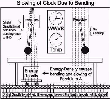
If a high, energy-density source can be found, then this new theory predicts that the diallel, gravitational-field lines radially protruding from the earth will be bent toward the vertical, center-line of this high, energy-density body, that is sitting on the earth.
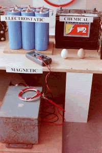
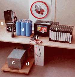
Two high-quality, nearly-identical, commercial pendulum clocks were employed for the experiment. They were placed on a low table and on either side of a reference clock and a thermometer. (See Figure 1) Later, we will also discuss the temperature effects on the experiment. The table was constructed sufficiently low so that the energy density source could be placed immediately under one clock (pendulum clock A) and then conveniently moved to be under the other clock (pendulum clock B) for an A, B comparison.
4.2 Time and Frequency Measurement TechniquesThough the apparatus was relatively simple and the experimental setup not complicated, the best time and frequency metrology techniques were implemented to ascertain the size of the effect and its uncertainty (see figure 1)[Allan]. Vastly superior techniques could have been designed and implemented to study the desired effect, but the resources were not readily available. The measurement equipment used, though rather primitive, was adequate to achieve the precision needed. 4.2.1 Advantage of Heterodyne TechniqueThe heterodyne principle was used in order to obtain additional leverage on the precision needed for the experiment. This was accomplished by designing a beat frequency between the two pendulums. From the equation above one can see that the period of the pendulum is dependent upon its length. The suspension on pendulum A was shortened slightly and the suspension on pendulum B was lengthened slightly. A beat period of 100 seconds was chosen for reasons that will be explained later. The period of the pendulums used was about 1.36 seconds, and for this period the length difference needed was about 12.5 millimeters for simple pendulums. To see the advantage of the heterodyne principle, let <A be the frequency of pendulum A and let <0 be the ideal reference frequency. We can write the fractional offset frequency of pendulum A as follows:
where <b is the beat or difference frequency. If we take the time derivative of equation (5), realizing also that <b = 1 / Tb , where Tb is the beat period, we obtain the following:
Hence, very small changes in the fractional frequency of pendulum A can be observed corresponding to much larger changes in the beat period as reduced by the heterodyne factor, <b /< 0 The heterodyne factor acts like an error multiplier -- making changes much easier to observe. In our case the heterodyne factor was about 1.35X10², or in terms of error multiplication it is about 74. 4.2.2 Counting Cycles of the PendulumsBecause these particular pendulum clocks did not have a mechanism for counting the number of swings that had occurred, this had to be done externally. Should there be any question about the number of cycles that had transpired, the experiment was videotaped. In worst-case, the number of cycles could be counted against the WWVB reference clock, that is tied to the Atomic Clock at NIST Boulder, Colorado. Fortunately, through some time and frequency metrology tricks this did not have to be done. Because of the good stability of the pendulum clocks, a few cycles could be measured precisely with a quartz crystal oscillator based stop watch, and then the occurrence of a future cycle could be predicted. This process was continued -- giving refinement in the measurement of the pendulums' beat period as the experiment progressed. [Sullivan] The beat period of 100 seconds, chosen above, gave both a useful heterodyne factor, and it also helped in resolving the counting of the correct number of cycles that had transpired. For example, every three beat periods (300 s or 5 minutes), the two pendulum clocks would come into synchronism again. The precise timing of the beat periods between the two pendulum clocks gave us the accuracy we needed to detect changes in the pendulum periods. 4.2.3 The Reference ClockThe WWVB clock has a radio receiver to keep it locked to the atomic clock in Boulder, Colorado. This radio receiver wakes up at 11:00 p.m. local time, and synchronizes the internal clock to the Boulder clock. We had three such clocks on site for this experiment. Even though the specification on the clocks was an accuracy of 0.8 seconds, the three clocks were typically in agreement within one or two tenths of a second. Frequency stability of the WWVB clock was estimated to be of the order of one part in 106. 4.2.4 The Quartz Stop WatchThe contribution of the stop watch to the measurement uncertainty was com-parable to that of the WWVB clock. This is because its time base was also a quartz crystal oscillator, and it was used strictly as a stop watch and not as a source of accurate time. In other words, it was used as an independent source of timing of the periods of the pendulums. The frequency stability of the quartz crystal oscillator in the stop watch was also estimated to be of the order of one part in 106. The readout of the stop watch was to 10 milliseconds. The main limitation for the stop watch measurement was the human reaction time -- ability to push the button at the right moment. This reaction time was tested to be at about 40 milliseconds using the WWVB clock as a calibration device. 4.2.5 Double the Precision with A,B ComparisonThe energy-density body was first placed directly under pendulum A and left for sufficient averaging time (typically an hour). Then, it was moved under pendulum B and left for the same amount of time -- then back under pendulum A, and this process was repeated N times. Let us assume that each time the energy-density is placed under a clock that the size of the frequency slowing of the clock is * -- according to the new theory. Let <A and <B be the natural un-perturbed frequencies of the two pendulums. Then we may write an expression for the fractional beat frequency when the energy density is under A and then under B:
Now if we observe the change in the fractional frequency between these two measurements, we may calculate yB - yA, which from the above equations yields:
So we see that we gain an additional factor of 2 in the precision using this technique. Further, we may approximate equation (6) with finite differences replacing the derivatives:
By combining the heterodyne principle with the A, B Comparison technique, we obtain an error multiplication factor of 2X74 = 148 for our experiment, which turned out to be very useful and sufficient. When no energy-density source was placed under either pendulum clock, then we simply observed, as expected, the random variations of the free-running clocks, but without the steps in frequency that occur coincident with the introduction of a high, energy-density source immediately below it. 4.2.6 Use of Synchronous Detection and AveragingOne of the significant limitations in many precision experiments is in dealing with drifts, trends, and low frequency processes such as 1/f noise and random-walk noise. These effects have no convergent variances and often degrade the precision otherwise obtainable. These limitations can, in large measure, be dealt with by using synchronous detection. In the above averaging time, the average is long enough to average down to
what is called the "flicker floor." This is where the frequency
stability versus averaging time J bottoms
out. At this nominal J value, we switch the
energy-density from under clock A to being under clock B. We wait another
interval J , then switch it back --
recording the change in beat period (per the above equation)
synchronous with these intervals. In a well controlled experiment, the changes
in frequency will have random and uncorrelated residuals. We tested ours for the
longest and most difficult part of the experiment with the trans-former, and
they were random and uncorrelated. In this case, the confidence on the estimate
of the size of the effect is the standard deviation of the mean. In other words,
the confidence improves as 5 Experimental ResultsWe tabulate below the experimental results of how much the pendulum clocks were slowed in parts in a million. We also list the confidence on the estimate per the above discussion and the number, N, of switches for each of the three different types of energy densities. There was some temperature dependence between the pendulum clocks. This was only a significant problem for the magnetic-field energy-density because of all the heat generated in order to properly load the 5 kilowatt transformer. From the above pendulum equation, as the length increases with increasing temperature, the period of the pendulum will increase. For brass, this is only about 10 parts in a million per degree centigrade. Since we were observing the differential by looking at the beat period, the effect should be smaller, but it was not. Apparently, the temperature effects upon the support and actuating mechanism was more significant. We measured a coefficient over a reasonably linear portion of the data, then subtracted, to first order, the effects of temperature from the data. The temperature was relatively stable for the other two energy-densities, since they dissipated negligible heat. The pendulum bob was tested as being made of magnetic material. Being concerned about the stray magnetic fields associated with the transformer coupling to the pendulum bob, a magnetic field coil sensor was constructed in order to find a transformer configuration where there would be negligible magnetic-field coupling to the pendulum bob. Such an orientation was successfully found, and we believe that any residual coupling had negligible effects on the results of the experiment. It is interesting that classical gravitational theory gives a speeding up of the pendulum by about one part in a billion due to the simple introduction of a mass under the pendulum. This is more than a thousand times smaller (hence, unmeasureable) and of opposite sign as can be calculated from equations (3) and (4) above than that given by the new theory.
Since the pendulum is only swinging, basically, in one dimension, and the energy-density diallel line configuration is theoretically a five-dimensional field system, one may expect the slowing to be proportional to the fifth power of the clock slowing. Well within the uncertainties of the measurement, the chemical and the electrostatic results, taken together, are consistent with this hypothesis. Though the dimension of time is also present, during each of the measurement periods, the diallel-lines were time independent and stationary. Hence, the effects of the time dimension were negligible. Within the experimental errors, a fourth power and a sixth power are consistent with the data, but the fifth power is by far the closest fit to the data -- as well as being consistent with the new theory. Clearly, this power law dependence and dimensionality needs to be studied with greater precision and in much more detail.
|
| |||||||||||||||||||||||||||||||||||||||||||||||||||||||||||||||||||||||||||||||||||||
|